Analyzing NFL Stats with Python

The dataset I worked with comprised of NFL game stats during the 2021 NFL season. They contained offensive and defensive stats for each game played by each team (including postseason games where applicable) as well as game details such as which teams are competing, the date of the matchup, and the outcome of the game.

First Step: Loading the Dataset

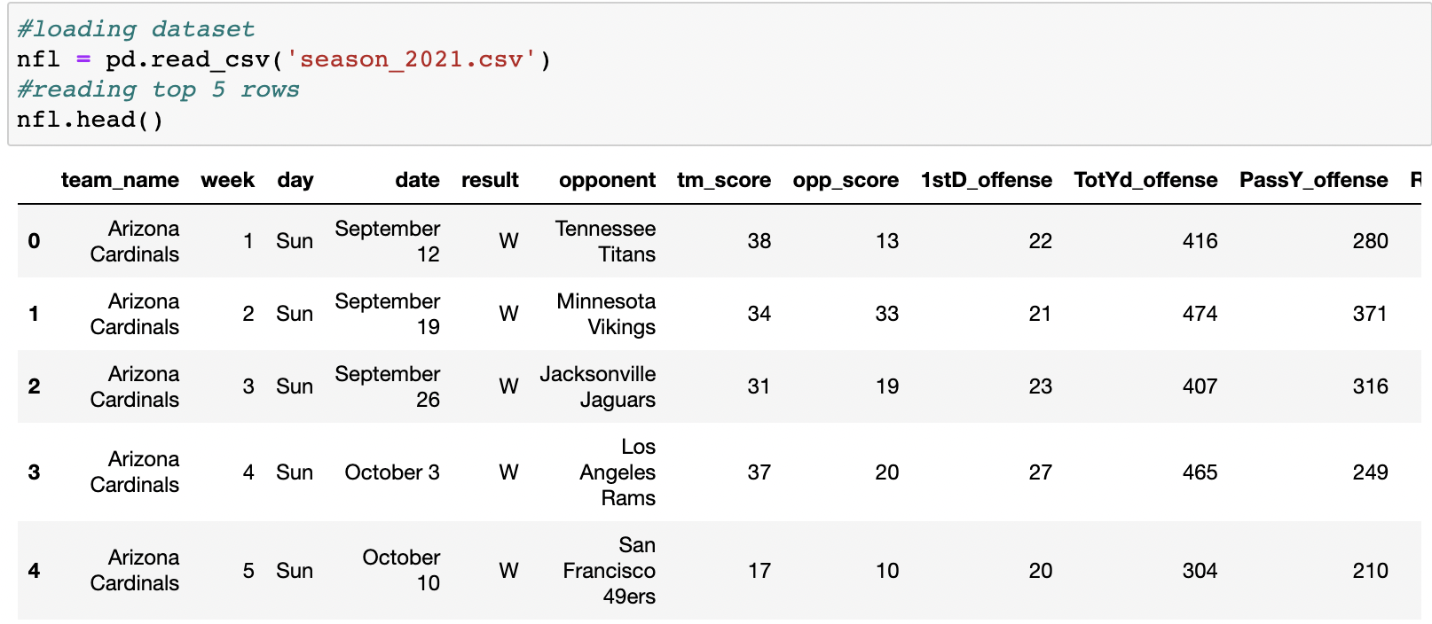
After importing the libraries I needed to perform my analysis, I loaded the dataset using the pandas command pd.read_csv(). To ensure that the dataset was loaded correctly, I used the .head() function to view the first 5 rows of the dataset.

Second Step: Summarizing and Encoding Outcomes

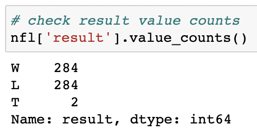
The next step was to count the number of wins and losses in the season and I did this by running the following line of code nfl['result'].value_counts() which counted each unique value in the results column.

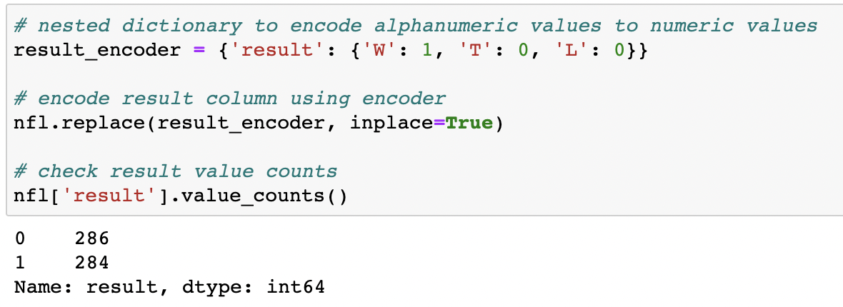
Since I was going to use a regression algorithm to predict future game outcomes, I needed to convert W,L,T into 1 and 0 in order for the algorithm to work. Since there are three outcomes, I combined the losses and ties together and created a nested library result_encoder = {'result': {'W': 1, 'T': 0, 'L': 0}} and used nfl.replace(result_encoder, inplace=True) to replace all the values in the results column. Finally, to check if my code worked, I ran the same code nfl['result'].value_counts() to count the results.

Third Step: Visualizing the Statistics

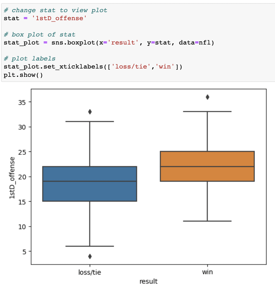
The next step was to explore trends in the stats would be used to predict wins. The variable stat has been set to 1stD_offense because the winning team typically has a higher number of first downs in a game.

I used sns.boxplot() to create a box plot of stat by wins and losses, and set the x, y, and data parameters inside the function and saved the plot as stat_plot. I set the x label of the graph to loss/tie and win by using .set_xticklabels([]).

After comparing first downs in winning games  to first downs in losing games, it can be assumed that the winning team typically has a higher number of first downs in a game. I changed the stat from 1stD_offense to other statistics, and through this I came to the conlusion that winning teams have higher offensive stats on average (indicating more opportunities to score points) and lower defensive stats on average (indicating fewer opportunities for the opponent to score points).

Fourth Step: Preparing the Data

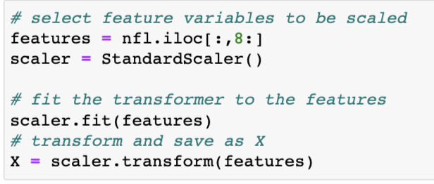
To prepare the data for the regression model . I first had to standardize the statistics in order to be able to compare them to one another and be able to improve the models accuracy in the future. I used the functions .fit() and .transfrom from the sklearn library to fit features to the scaling function and standardize the game stats. I saved the the output to X.

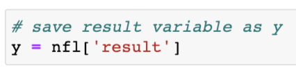
For easier reference, I also saved the game outcome variable to y using the line of code above.

The final step I took to prepare the data for the model was to split the data into training and testing data. Using the train_test_split() function from the sklearn library, I was able to split the data in half at random. The training data was saved to X_train and y_train, and the testing data was saved to y_train and y_test.

Fifth Step: Analyzing the Data

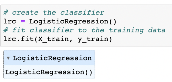
In this step I trained my model to use the patterns of the offensive and defensive stats to predict the probability of a winning game. I created a LogisticRegression() classifier and saved it to the variable lrc. Then called the .fit() function using the training data X_train and y_train.

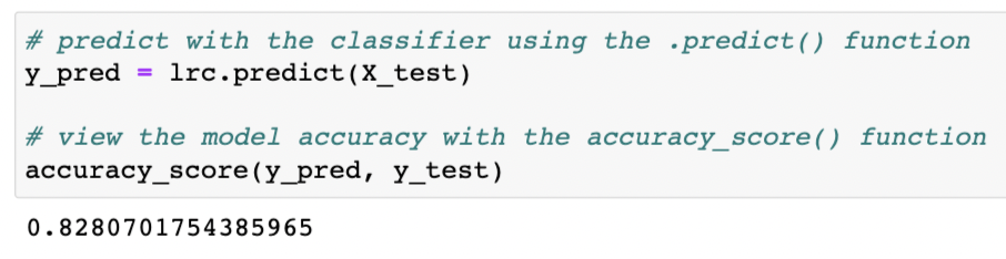
With the classifier fitted to the training data, I used the trained classifier to make predictions on the test data. I passed the test features X_test as a parameter of lrc.predict() and saved the resulting predictions as y_pred.

I checked the percentage of outcomes that my model predicted correctly. I used the accuracy_score() function imported from the sklearn library to compare my predicted test values y_pred to the true values y_test.

I noticed from the model performance that the model can predict wins and losses with good accuracy. My model correctly predicted the game outcome for 82.8% of the games in the test set.

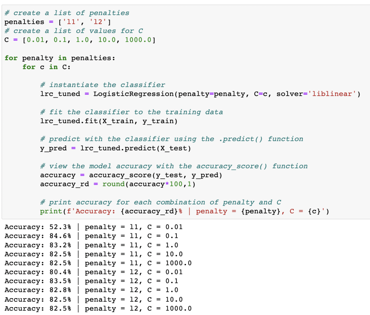
I could improve the model performance by closely studying how different paremeters affect performance. I considered two hyperparameters for the LogisticRegression classifer: penalty and C. After running the code above to test out different penatly and c values, I concluded that a lot of these accuracy scores are very similar to the original accuracy score. The model gained a small benefit by changing the hyperparameters to penalty = l1 and C = 0.1. The change increased the accruacy from 82.8% to 84.6%.

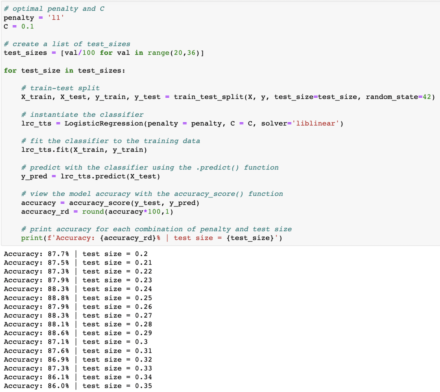
Since changing the penalty and c values only slightly improved the accuracy of the model, I tried to optimize the test size to see if it would affect the accuracy in a positive manner. As you can see from the output, I was able to improve accuracy slightly with a test size of 0.25. I was able to improve the accuracy from 84.6% to 88.8%.

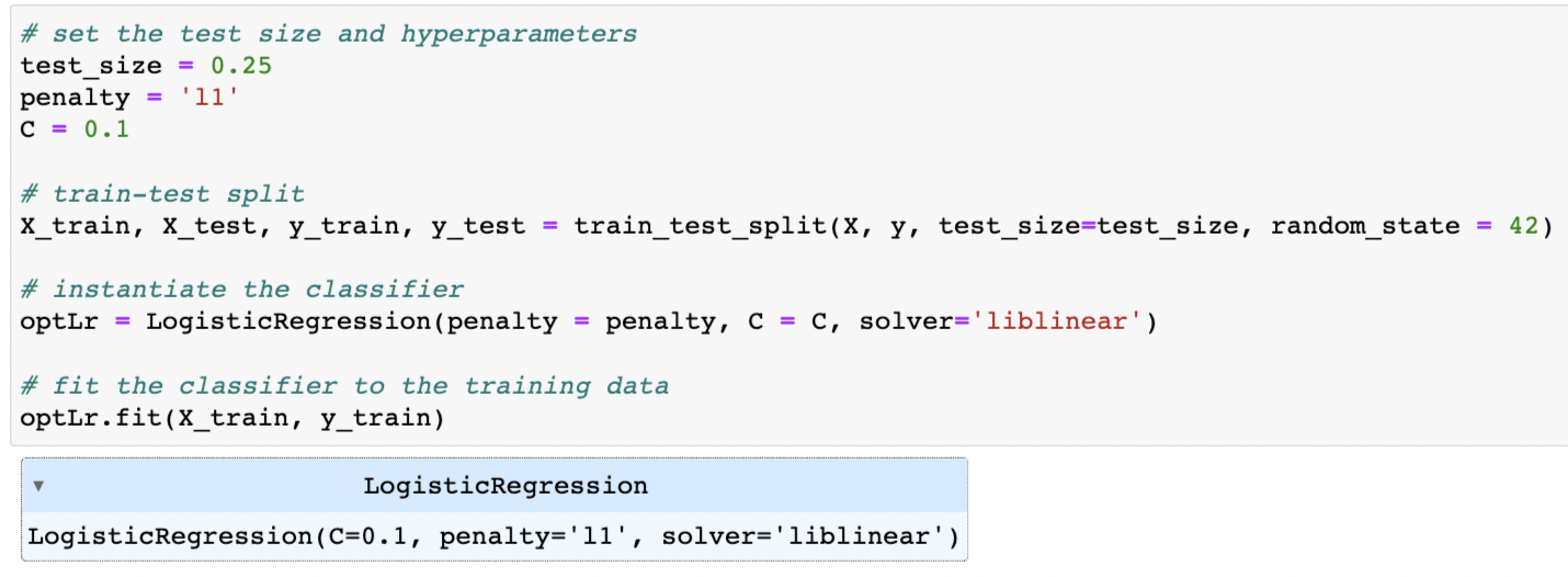
After figuring out the optimal parameters for the model, I ran and saved the final model with the optimal choices for test_size, penalty, and C and kept random_state = 42.

Sixth Step: Analyzing Feature Importance

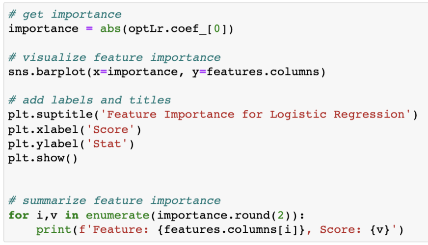
I used the code above to save the absolute values of the model coefficient to importance and create a bar plot of the feature importance which you can see below.

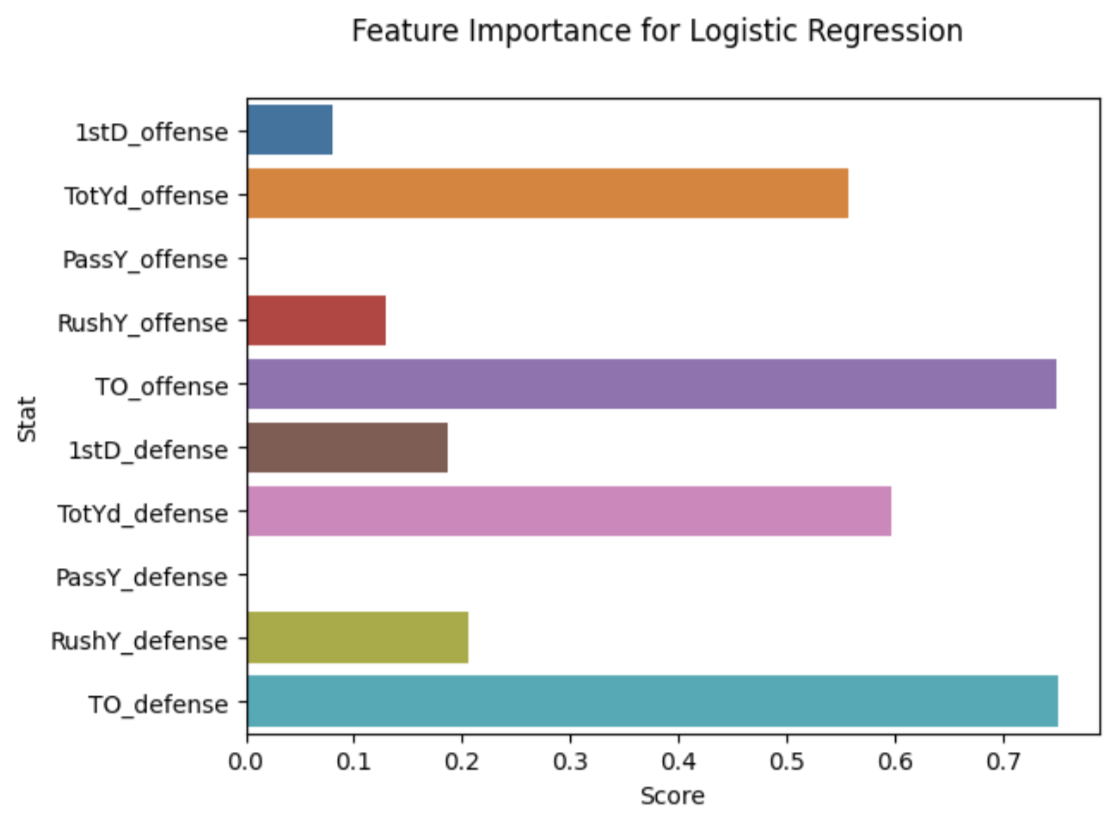
It looks like the most important stats in our model were turnovers: TO_offense and TO_defense both had much larger importance scores than the other stats. After that, total yards were the next most influential stats.